![]()
INTRODUCTION |
You make a hypothesis (called the null hypothesis), for example to check if the coin lying in front of you is not a fake, which means that the probability for landing on heads and tails is the same (p = ½). Or, you might have a die in front of you and make a hypothesis that it is not loaded, which means that all 6 numbers have the same probability of occurring (p = 1/6). In this chapter you will learn a method to test your hypothesis, however not with absolute certainty as you assume a 5% probability (significance level) with which the null hypothesis is wrongly rejected. |
A SIGNIFICANTLY FAKE COIN |
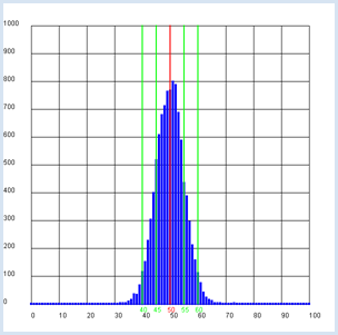
You begin with the null hypothesis that the coin is not a fake and if you toss it n = 100 times, you get heads a certain number of times k and tails n - k times.
If you mark the area corresponding to 95% of all cases, you obtain approximately double the dispersion (here between 40 and 60). from gpanel import * from random import random n = 100 # size of the test group p = 0.5 z = 10000 def showDistribution(): setColor("blue") lineWidth(4) for t in range(n + 1): line(t, 0, t, h[t]) def showMean(): global mean count = 0 for t in range(n + 1): count += h[t] * t mean = int(count / z + 0.5) setColor("red") lineWidth(2) line(mean, 0, mean, 1000) text(mean - 1, -30, str(mean)) def showSpreading(level): count = h[mean] for s in range(1, 20): count += h[mean + s] + h[mean - s] if count > z * level: break setColor("green") lineWidth(2) line(mean + s, 0, mean + s, 1000) text(mean + s - 1, -30, str(mean + s)) line(mean - s, 0, mean - s, 1000) text(mean - s - 1, -30, str(mean - s)) def sim(): count = 0 repeat n: w = random() if w < p: count +=1 return count makeGPanel(-0.1 * n, 1.1 * n, -100, 1100) title("Coin toss, distribution of number") drawGrid(0, n, 0, 1000) h = [0] * (n + 1) repeat z: k = sim() h[k] += 1 showDistribution() showMean() showSpreading(0.68) showSpreading(0.95)
|
MEMO |
|
If you frequently make a test with 100 coins that are not fake, in 68 % of all cases the number of tossed heads lies in the area 50 +-5, and 95% of all cases in the area 50 +-10 [more...
The theoretically calculated value is If you make a test with the coin that is lying in front of you and you get a value for the number of heads that is greater than 60 or smaller than 40 you reject the hypothesis that the coin is not fake, in other words, you say that the coin is fake. In this case, you may be mistaken with a probability of 5% (the significance level). Sometimes you can also concisely say that the present coin is significantly fake. |
A SIGNIFICANTLY LOADED DIE |
You have a die in front of you and want to test whether it is a fair die, which means that all numbers can occur with the same probability of 1/6. You make the hypothesis: The die is not loaded. Here you will get to know a slightly different method from one that we used with the coin since there are six, not only two, possibilities that can occur on a roll, namely the numbers from 1 to 6. To be on the safe side you will want to roll the die often, let's say around 600 times, and write down the frequencies of the numbers that occur.
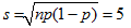
Observed and theoretical frequencies In order to introduce a measure for the deviation of the observed from the theoretical occurrences, you need to calculate the relative square deviation for each number (u - e)2 / eand add up these values. We call the result χ2 (pronounced "Chi-square").
from gpanel import *
from random import random, randint

n = 600 # number of tosses
p = 1 / 6
z = 10000

def showDistribution():
    setColor("blue")
    lineWidth(4)
    for i in range(21):
        line(i, 0, i, h[i])

def showLimit(level):
    count = 0
    for i in range(21):
        count += h[i]
        if count > z * level:
            break
    setColor("green")
    lineWidth(2)
    line(i, 0, i, 2000)
    text(i, -80, str(i))
    return i

def chisquare(u):
    chi = 0
    e = n * p
    for i in range(1, 7):
        chi += ((u[i] - e) * (u[i] - e)) / e
    return chi

def sim():
    u = [0] * 7
    repeat n:
        t = randint(1, 6)
        u[t] += 1
    return chisquare(u)

makeGPanel(-2, 22, -200, 2200)
title("Chi-square simulation  is being carried out. Please wait...")
drawGrid(0, 20, 0, 2000)
h = [0] * 21

repeat z:
    c = int(sim())
    if c < 20:
        h[c] += 1
    else:
        h[20] += 1

title("Chi-square test on  the die")
showDistribution()
s = showLimit(0.95)

# Observed series
u1 = [0, 112, 128, 97, 103, 88, 72]
u2 = [0, 112, 108, 97, 113, 88, 82]
c1 = chisquare(u1)
c2 = chisquare(u2)
print("Die with", u1, "Xi-square:", c1, "loaded?", c1 > s)
print("Die with", u2, "Xi-square:", c2, "loaded?", c2 > s)
|
MEMO |
|
The computer simulation exposes the following result: in 95% of all cases, χ2 is less than or equal to the critical value 11. Hence, you have found a method to test if your die is rigged: calculate χ2 from the observed frequency. If the value is greater than 11, you can say with a 5% probability of being wrong that your null hypothesis of it being a fair die is incorrect, and therefore the die is loaded. The frequencies of the table above result in χ2 = 18.7. In other words, the die has a very high probability of being loaded. With another die rolled 600 times you get the frequencies u2 = [112, 108, 97, 113, 88, 82]. Since you obtain χ2 = 8.5, there is a low probability that the die is loaded. |
DIFFERENCES IN HUMAN BEHAVIOR |
You can also apply the χ2 test to a study of the behavior of two groups of people. An interesting question often asked is whether in a particular context the behavior of females and males should be appraised to be statistically different, or whether both sexes behave equally. You assume that the use of Facebook is studied in a secondary school. A total of 106 girls (women) and 86 boys (men) were asked whether they have a Facebook account. The survey results are as follows:
The percentage of people who have a Facebook account is substantially greater among females than it is with males. But it raises the question of whether this higher proportion is statistically significant.
You must now still determine the expected value e for all four cases. You can assume that p = (f0 + m0) / n is the total probability for a Yes and correspondingly 1 - p is the total probability for a No, so you calculate:
The rest of the program remains largely unchanged from the die test. from gpanel import * from random import random z = 10000 # survey values/polls females_yes = 87 females_no = 19 males_yes = 62 males_no = 24 def showDistribution(): setColor("blue") lineWidth(4) for i in range(101): line(i/10, 0, i/10, h[i]) def showLimit(level): count = 0 for i in range(101): count += h[i] if count > level * z: break setColor("green") lineWidth(2) limit = i / 10 line(limit, 0, limit, 1000) text(limit, -80, str(limit)) return limit def chisquare(f0, f1, m0, m1): # f: females, m: males, 0:yes, 1:no w = (f0 + m0) / n # probability of a yes # expected value ef0 = (f0 + f1) * w # females-yes em0 = (m0 + m1) * w # males-yes ef1 = (f0 + f1) * (1 - w) # females-no em1 = (m0 + m1) * (1 - w) # males-no # add up deviations (u - e)*(u - e) / e chi = (f0 - ef0) * (f0 - ef0) / ef0 \ + (m0 - em0) * (m0 - em0) / em0 \ + (f1 - ef1) * (f1 - ef1) / ef1 \ + (m1 - em1) * (m1 - em1) / em1 return chi def sim(): # simulate females f0 = 0 # yes f1 = 0 # no for i in range(females_all): t = random() if t < p: f0 += 1 else: f1 += 1 # simulate males m0 = 0 # yes m1 = 1 # no for i in range(males_all): t = random() if t < p: m0 += 1 else: m1 += 1 return chisquare(f0, f1, m0, m1) females_all = females_yes + females_no males_all = males_yes + males_no n = females_all + males_all # all p = (females_yes + males_yes) / n # probability of yes for all print("Facebook yes (all):", round(100 * p, 1), "%") pf = females_yes / females_all print("Facebook yes (females):", round(100 * pf, 1), "%") pm = males_yes / males_all print("Facebook yes (males:)", round(100 * pm, 1), "%") makeGPanel(-1, 11, -250, 2750) title("Chi-square test, use of Facebook") drawGrid(0, 10, 0, 2500) h = [0] * 101 repeat z: c = int(10 * sim()) # magnification factor of 10 if c < 100: h[c] += 1 else: h[100] += 1 showDistribution() s = showLimit(0.95) c = chisquare(females_yes, females_no, males_yes, males_no) print("critical value:", s) print("observed:", c) if c <= s: print("- the same behavior") else: print("- not the same behavior")
|
MEMO |
|
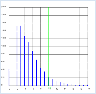
The result is astonishing: the χ2significance limit is 3.8 [more... The value corresponds to the value of the χ2 table for 1 degree of freedom a significance of 0.95]. The survey values resulted in the smaller value of 2.7. Even though the proportion of females with accounts is essentially higher, it cannot be statistically proven that they differ substantially from the males with respect to Facebook. |
EXERCISES |
|