8.7 COMPLEX NUMBERS & FRACTALS
![]()
INTRODUCTION |
Complex numbers are very important in mathematics since they extend the set of real numbers allowing many propositions to be formulated easier and more general. They also play an important role in science and technology, especially in physics and electrical engineering [more...
Quantum mechanics is based entirely on complex numbers and, in the field of electrical Complex numbers can be represented in the complex plane as arrows or as points. In order to allow that turtle windows, GPanels, and JGameGrid pixel grids can also be regarded as a complex planes, all functions with coordinate parameters (x,y) in the respective libraries are also directly available for complex numbers. |
BASIC OPERATIONS WITH COMPLEX NUMBERS |
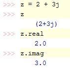
In Python, for the imaginary unit you use the symbol j commonly seen in electrical engineering instead of i. You can define the complex number with the real part 2 and the imaginary part 3 in several ways:
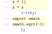
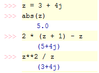
Use the convenient TigerJython console for the following examples:
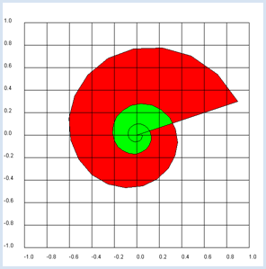
from gpanel import *
makeGPanel(-1.2, 1.2, -1.2, 1.2)
title("Complex plane")

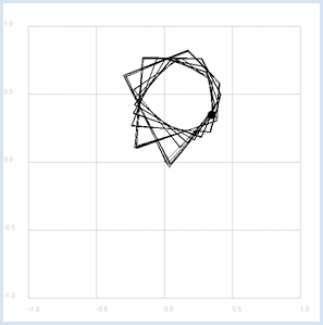
z = 0.9 + 0.3j
for n in range(1, 60):
    y = z**n
    draw(y)
fill(0.2, 0, "white", "red")
fill(0.0, 0.2, "white", "green")
drawGrid(-1.0, 1.0, -1.0, 1.0)
|
MEMO |
|
draw(z) causes the same as draw(z.real, z.imag), but it is simpler. You should use GPanel coordinates that are 10% larger on all sides than the used coordinate range. You must specify the coordinates as floats in drawGrid() so that the grid is labeled with floats. |
CONFORMAL MAPPING |
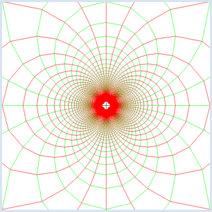
In a two-dimensional mapping every point P(x, y) is assigned a pixel P'(x', y').
from gpanel import *

# function f(z) = 1/z
def f(z):
    if z == 0:
        return 0
    return 1 / z

min_value = -5.0
max_value = 5.0
step = 1 / 20
reStep = complex(step, 0)
imStep = complex(0, step)

makeGPanel(min_value, max_value, min_value, max_value)
title("Conformal mapping for f(z) = 1 / z")
line(min_value, 0, max_value, 0)  # Real axis
line(0, min_value, 0, max_value) # Imaginary axis

# Transform horizontal line per line
setColor("green")
z = complex(min_value, min_value)
while z.imag < max_value:
    z = complex(min_value, z.imag) # left
    move(f(z))
    while z.real < max_value: # move along horz. line
        draw(f(z))
        z = z + reStep
    z = z + imStep

# Transform vertical line per line
setColor("red")
z = complex(min_value, min_value)
while z.real < max_value:
    z = complex(z.real, min_value) # bottom
    move(f(z))
    while z.imag < max_value:  # move along vert. line
        draw(f(z))
        z = z + imStep
    z = z + reStep
|
MEMO |
|
What you can gather from the picture is that the images of the grid lines still intersect perpendicularly. A mapping where the angles between intersecting lines is maintained is called conformal and so we speak of a conformal mapping [more... It can be proved mathematically precise that the inversion is a conformal mapping] . |
MANDELBROT FRACTALS |
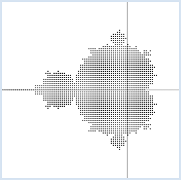
To generate a Mandelbrot fractal you look at a (recursively defined) sequence of complex numbers for the given complex number c according to the formation rule
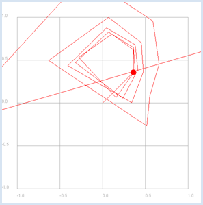
If the amount of the sequence terms remains in a confined area, meaning that they do not grow beyond all limits, c belongs to the Mandelbrot set. To familiarize yourself with the algorithm, you draw the following terms for two complex numbersc1 = 0.35 + 0.35j and c2 = 0.36 + 0.36j. You will immediately see that c1 belongs to the Mandelbrot set, but c2 does not.
from gpanel import *

def f(z):
    return z * z + c

makeGPanel(-1.2, 1.2, -1.2, 1.2)
title("Mandelbrot iteration")

drawGrid(-1, 1.0, -1, 1.0, 4, 4, "gray")

isMandelbrot = askYesNo("c in Mandelbrot set?")
if isMandelbrot:
    c = 0.35 + 0.35j
    setColor("black")
else:
    c = 0.36+ 0.36j
    setColor("red")

title("Mandelbrot iteration with c = " + str(c))
move(c)
fillCircle(0.03)

z = 0j
while True:
    if z == 0:
        move(z)
    else:
        draw(z)
    z = f(z)
    delay(100)
from gpanel import *

def isInSet(c):
    z = 0
    for n in range(maxIterations):
        z = z*z + c
        if abs(z) > R: # diverging
            return False
    return True

maxIterations = 50
R = 2
xmin = -2
xmax = 1
xstep = 0.03
ymin = -1.5
ymax = 1.5
ystep = 0.03

makeGPanel(xmin, xmax, ymin, ymax)
line(xmin, 0, xmax, 0)  # real axis
line(0, ymin, 0, ymax) # imaginary axis
title("Mandelbrot set")
y = ymin
while y <= ymax:
    x = xmin
    while x <= xmax:
        c = x + y*1j
        inSet = isInSet(c)
        if inSet:
            move(c)
            fillCircle(0.01)
        x += xstep
    y += ystep
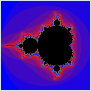
from gpanel import * def getIterationColor(it): color = makeColor((30 * it) % 256, (4 * it) % 256, (255 - (30 * it)) % 256) return color def mandelbrot(c): z = 0 for it in range(maxIterations): z = z*z + c if abs(z) > R: # diverging return it return maxIterations maxIterations = 50 R = 2 xmin = -2 xmax = 1 xstep = 0.003 ymin = -1.5 ymax = 1.5 ystep = 0.003 makeGPanel(xmin, xmax, ymin, ymax) title("Mandelbrot set") enableRepaint(False) y = ymin while y <= ymax: x = xmin while x <= xmax: c = x + y*1j itCount = mandelbrot(c) if itCount == maxIterations: # inside Mandelbrot set setColor("black") else: # outside Mandelbrot set setColor(getIterationColor(itCount)) point(c) x += xstep y += ystep repaint() |
MEMO |
|
To speed up the drawing, you set enableRepaint(False) and only re-render at the end of each line using repaint(). The Mandelbrot fractal possesses the remarkable feature that when a section is magnified, a similar structure appears [more... However, the structure is not exactly the same and in this fractal is not strictly self-similarh] . |
EXERCISES |
|
ADDITIONAL MATERIAL |
ALTERNATING CURRENT AND IMPEDANCE |
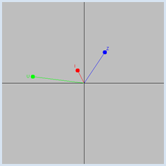
Electrical circuits for sinusoidal alternating voltages and alternating currents, which are built from passive devices (resistors, capacitors, inductors), can be treated like direct current circuits if you are using complex variables for voltages, currents, and resistors. A general complex resistor is also called an impedance and is often denoted with Z (and for purely imaginary resistors, X). The impedance of an ohmic resistor is R, of an inductor is XL = jωL (L: inductance) and of a capacitor is XC = 1 / jωC (C: capacitance), where ω = 2πf (f: frequency). A complex alternating voltage u = u(t) runs uniformly on a circle in the complex plane. If it is applied to an impedance Z, the current i(t) flows according to Ohm's law u = Z * i. Since in complex multiplication the phases are added and the absolute values multiplied, u runs before i, phase-shifted by the phase of Z
So, i also runs on a circle. The following absolute values (amplitudes) we have:
from gpanel import *
import math

def drawAxis():
   line(min, 0, max, 0)  # real axis
   line(0, min, 0, max) # imaginary axis


def cdraw(z, color, label):
    oldColor = setColor(color)
    line(0j, z)
    fillCircle(0.2)
    z1 = z + 0.5 * z / abs(z) - (0.1 + 0.2j)
    text(z1, label)
    setColor(oldColor)

min = -10
max = 10
dt = 0.001

makeGPanel(min, max, min, max)
enableRepaint(False)
bgColor("gray")
title("Complex voltages and currents")

f = 10 # Frequency
omega = 2 * math.pi * f

t = 0
uA = 5
Z = 2 + 3j

while True:
    u = uA * (math.cos(omega * t) + 1j * math.sin(omega * t))
    i = u / Z
    clear()
    drawAxis()
    cdraw(u, "green", "U")
    cdraw(i, "red", "I")
    cdraw(Z, "blue", "Z")
    repaint()
    t += dt
    delay(100)
|
MEMO |
|
Electrical circuits with passive devices can be treated as direct current circuits if you regard voltage, current, and resistance as complex numbers. |
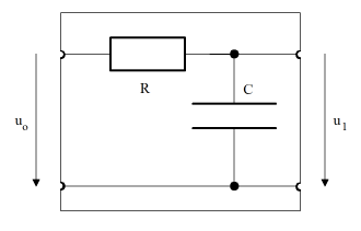
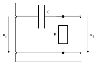
The calculation is simple: The series circuit of R and C results in the impedance Z = R + XC and thus the current i = uo / Z, so again using Ohm's law the output voltage
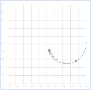
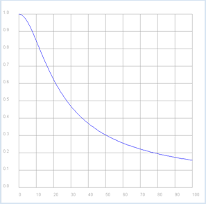
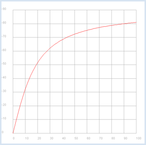
from gpanel import * from math import pi def drawAxis(): line(-1, 0, 1, 0) # Real axis line(0, -1, 0, 1) # Imaginary axis makeGPanel(-1.2, 1.2, -1.2, 1.2) drawGrid(-1.0, 1.0, -1.0, 1.0, "gray") setColor("black") drawAxis() title("Complex gain factor – low pass") R = 10 C = 0.001 def v(f): if f == 0: return 1 + 0j omega = 2 * pi * f XC = 1 / (1j * omega * C) return XC / (R + XC) f = 0 # Frequency while f <= 100: if f == 0: move(v(f)) else: draw(v(f)) if f % 10 == 0: text(str(f)) f += 1 delay(10) The gain factor in the Bode plot is divided by magnitude and phase, and plotted in function of the frequency (logarithmic scales are commonly used).
from gpanel import * import math import cmath R = 10 C = 0.001 def v(f): if f == 0: return 1 + 0j omega = 2 * math.pi * f XC = 1 / (1j * omega * C) return XC / (R + XC) p1 = GPanel(-10, 110, -0.1, 1.1) drawPanelGrid(p1, 0, 100, 0, 1.0, "gray") p1.title("Bode Plot - Low Pass, Gain") p1.setColor("blue") f = 0 while f <= 100: if f == 0: p1.move(f, abs(v(f))) else: p1.draw(f, abs(v(f))) f += 1 p2 = GPanel(-10, 110, 9, -99) drawPanelGrid(p2, 0, 100, 0, -90, 10, 9, "gray") p2.title("Bode Plot - Low Pass, Phase") p2.setColor("red") f = 0 while f <= 100: if f == 0: p2.move(f, math.degrees(cmath.phase(v(f)))) else: p2.draw(f, math.degrees(cmath.phase(v(f)))) f += 1 |
MEMO |
|
The Bode-Plot once again particularly clarifies that the present circuit transmits low frequencies well and high frequencies poorly. Additionally, a phase shift exists between the input and the output signal in the range of 0 to -90 degrees. |
EXERCISES |
|
