8.10 RANDOM WALK
![]()
INTRODUCTION |
Many phenomena are determined by chance in daily life and you often have to make decisions based on probabilities. For example, you may decide whether you should select one mode of transport over the other based on their probability of being involved in an accident. In such situations, the computer can be an important tool with which you can examine potential dangers using simulations, without actually risking anything. In the following, you assume that you got lost and can no longer find your way home. Thereby you observe a movement, called Random Walk, that happens at single time intervals where steps of equal length are chosen in a random direction. Even though such a movement does not necessarily correspond to reality, you get to know important characteristics that can be later applied to real systems, for instance the modeling of the stock market in financial mathematics, or the displacement of molecules. |
ONE-DIMENSIONAL RANDOM WALK |
Once again, turtle graphics is helpful in representing the simulation graphically. At time 0, the turtle is located at the position x = 0 and move along the x-axis at steps of equal length. At each step of time, the turtle "decides" whether to make a step to the left or to the right. In your program, it decides on one of the two options with the same probability p = ½ (symmetric random walk).
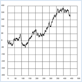
from gturtle import * from gpanel import * from random import randint makeTurtle() makeGPanel(-50, 550, -480, 480) windowPosition(880, 10) drawGrid(0, 500, -400, 400) title("Mean distance versus time") lineWidth(2) setTitle("Random Walk") t = 0 while t < 500: if randint(0, 1) == 1: setHeading(90) else: setHeading(-90) forward(10) x = getX() draw(t, x) t += 1 print("All done") |
MEMO |
You are probably surprised that, in most cases, the turtle gradually moves away from the starting point even though it makes every step, either a left or a right one, with the same likelihood. In order to investigate this important result more closely, your next program will determine the average distance d from the starting point after t steps in 1,000 walks. |
THE SQUARE ROOT OF TIME RULE |
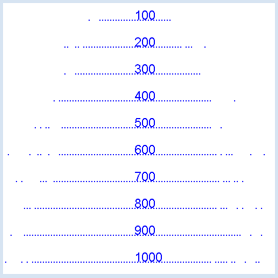
Repeat the simulation 1,000 times with a certain number of steps t at the fixed y position and draw the end position as a point. In order to speed up the results, you can hide the turtle and avoid drawing any traces. With every simulation experiment, you determine a distance r of the ending point from the starting point. For each set of experiments with a certain t, you will get an average distance d of the distances r, which you mark in a GPanel graphic. from gturtle import * from gpanel import * from math import sqrt from random import randint makeTurtle() makeGPanel(-100, 1100, -10, 110) windowPosition(850, 10) drawGrid(0, 1000, 0, 100) title("Mean distance versus time") ht() pu() for t in range(100, 1100, 100): setY(250 - t / 2) label(str(t)) count = 0 repeat 1000: repeat t: if randint(0, 1) == 1: setHeading(90) else: setHeading(-90) forward(2.5) dot(3) r = abs(getX()) count += r setX(0) d = count / 1000 print("t =", t, "d =", d, "q = d / sqrt(t) =", d / sqrt(t)) draw(t, d) fillCircle(5) print("all done")
|
MEMO |
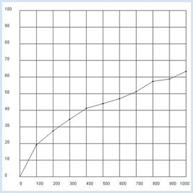
As you can see in the graphic visualization, the average value of the distance from the starting point grows with an increasing step size and time t. In the console, you also calculate the quotient q = d / sqrt(t). Because it is almost constant, the assumption suggests that d = q * sqrt(t) holds exactly, or: The average distance to the starting point increases by the square root of time. |
DRUNKEN MAN'S WALK |
It gets even more exciting once the turtle can move in two directions. This is called a two-dimensional random walk. The turtle always still makes the same length of steps, but each step is taken towards a random direction.
from gturtle import * from gpanel import * from math import sqrt makeTurtle() makeGPanel(-100, 1100, -10, 110) windowPosition(850, 10) drawGrid(0, 1000, 0, 100) title("Mean distance versus time") ht() pu() for t in range(100, 1100, 100): count = 0 clean() repeat 1000: repeat t: fd(2.5) setRandomHeading() dot(3) r = math.sqrt(getX() * getX() + getY() * getY()) count += r home() d = count / 1000 print("t =", t, "d =", d, "q = d / sqrt(t) =", d / sqrt(t)) draw(t, d) fillCircle(5) delay(2000) print("all done") |
MEMO |
The square root of time rule also applies for two-dimensional situations. In 1905, no less a person than Albert Einstein proved this rule for gas particles in his famous essay "On the Movement of Small Particles Suspended in Stationary Liquids Required by the Molecular-Kinetic Theory of Heat" and thus,provided us with a theoretical explanation of the Brownian motion. One year later, M. Smoluchowski had a different idea but came to the same results. |
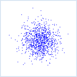
BROWNIAN MOVEMENT |
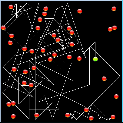
As early as 1827, the biologist Robert Brown had observed through a microscope that pollen grains in a drop of water make irregular twitching movements. He suspected an inherent vigor in the pollen. It was not until the discovery of the molecular structure of matter, that it became clear the thermal motion of water molecules colliding with the pollen are responsible for the phenomenon. Brownian motion can be nicely demonstrated in a computer simulation where the molecules are modeled as small spheres that swap velocities in collisions. The simulation can be easily implemented using JGameGrid because you can regard a particle collision as an event. To do this, you derive the class CollisionListener from GGActorCollisionListener and implement the callback collide(). You add each particle to the listener using addActorCollisionListener(). You may set the type and size of the collision area with setCollisionCircle(). For simplicity the 40 particles are arranged into 4 groups of velocities.
from gamegrid import * # =================== class Particle ==================== class Particle(Actor): def __init__(self): Actor.__init__(self, "sprites/ball.gif", 2) # Called when actor is added to gamegrid def reset(self): self.oldPt = self.gameGrid.toPoint(self.getLocationStart()) def advance(self, distance): pt = self.gameGrid.toPoint(self.getNextMoveLocation()) dir = self.getDirection() # Left/right wall if pt.x < 5 or pt.x > w - 5: self.setDirection(180 - dir) # Top/bottom wall if pt.y < 5 or pt.y > h - 5: self.setDirection(360 - dir) self.move(distance) def act(self): self.advance(3) if self.getIdVisible() == 1: pt = self.gameGrid.toPoint(self.getLocation()) self.getBackground().drawLine(self.oldPt.x, self.oldPt.y, pt.x, pt.y) self.oldPt.x = pt.x self.oldPt.y = pt.y # =================== class CollisionListener ========= class CollisionListener(GGActorCollisionListener): # Collision callback: just exchange direction and speed def collide(self, a, b): dir1 = a.getDirection() dir2 = b.getDirection() sd1 = a.getSlowDown() sd2 = b.getSlowDown() a.setDirection(dir2) a.setSlowDown(sd2) b.setDirection(dir1) b.setSlowDown(sd1) return 10 # Wait a moment until collision is rearmed # =================== Global section ==================== def init(): collisionListener = CollisionListener() for i in range(nbParticles): particles[i] = Particle() # Put them at random locations, but apart of each other ok = False while not ok: ok = True loc = getRandomLocation() for k in range(i): dx = particles[k].getLocation().x - loc.x dy = particles[k].getLocation().y - loc.y if dx * dx + dy * dy < 300: ok = False addActor(particles[i], loc, getRandomDirection()) # Select collision area particles[i].setCollisionCircle(Point(0, 0), 8) # Select collision listener particles[i].addActorCollisionListener(collisionListener) # Set speed in groups of 10 if i < 10: particles[i].setSlowDown(2) elif i < 20: particles[i].setSlowDown(3) elif i < 30: particles[i].setSlowDown(4) # Define collision partners for i in range(nbParticles): for k in range(i + 1, nbParticles): particles[i].addCollisionActor(particles[k]) particles[0].show(1) w = 400 h = 400 nbParticles = 40 particles = [0] * nbParticles makeGameGrid(w, h, 1, False) setSimulationPeriod(10) setTitle("Brownian Movement") show() init() doRun() |
MEMO |
The molecules are modeled in the class Particle which is derived from Actor. They have two sprite images, one red and one green for a specially distinguished molecule whose path you are tracking. The green image corresponds to the spriteID = 1 which you test in act() to draw the trail with drawLine(). |
EXERCISES |
|